A Quadrillion Rows across three Clouds: scaling LogHouse

LogHouse, our internal logging platform for ClickHouse Cloud, now stores 431 PiB of uncompressed data across 1.59 quadrillion rows. It spans 30+ regions across three cloud providers, and a typical query against any of them comes back in a few hundred milliseconds.

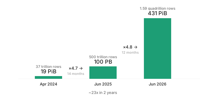
This is the third post in a series. In the first, we built LogHouse and replaced Datadog, at 19 PiB. In the second, we crossed 100 PB and introduced SysEx, our purpose-built pipeline for system-table telemetry that now sits alongside OpenTelemetry in our stack. Together, the three posts trace a steep curve: 19 PiB → 431 PiB, a 23x jump in two years, and 37 trillion → 1.59 quadrillion rows.

Introduction

Two years ago, the architecture was simple: one ClickHouse instance per region, and whoever needed logs connected to that region directly. That was fine at 19 PiB on a handful of AWS regions. It doesn't hold at 431 PiB across 30+.

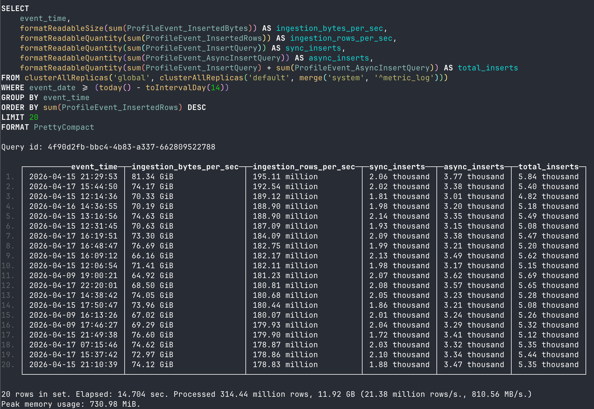
The pressure came from the write path first. As ClickHouse Cloud has grown, so has the volume of data flowing through it, reaching peaks of 80 GiB/s and 190 million rows per second. To keep pace, the write path needed to do two things well: scale horizontally and remain reliable while doing it.

The answer to the first challenge is geosharding. Writes stay local to the region where they arrive, avoiding cross-region egress costs and allowing each region to scale independently. As demand grows, busy regions can have multiple cells, providing near-linear scaling without affecting the rest of the system.

The catch is that while geosharding is a write-side decision, it incurs a read-side bill. Even with one cell per region, the per-region data source model was already awkward to manage and to use. Cells would have made it untenable. We weren't willing to push that complexity onto the people querying LogHouse.

So we set out to reconcile the two sides: let writes split as freely as we want, while making reads behave as if the topology underneath didn't exist. The rest of this post is about how we did that: first, the write path; then the read layer that makes cell creation transparent; and finally, the scaling limits we're beginning to run into next.

The numbers: A quadrillion rows

Today, LogHouse stores 431 PiB of uncompressed data across 1.59 quadrillion rows (1.59 × 10¹⁵). That's roughly a 23x increase from where we were two years ago.

System

Uncompressed Size

Rows

SysEx

335 PiB

1.48 quadrillion

OTel

95 PiB

109 trillion

Total

431 PiB

1.59 quadrillion

SysEx (responsible for exporting ClickHouse system tables) accounts for 78% of the volume and 93% of the rows, which is a clear validation of the architectural bet we described in our previous post. OpenTelemetry continues to handle stdout/stderr collection at info-level and above, serving as a safety net for crash-looping services where SysEx can't scrape system tables.

All 431 PiB compresses down to 27 PiB on disk, for roughly a 16x compression ratio - consistent with what we've seen since the early days of LogHouse. Most tables are retained for 180 days, with many SysEx tables kept for up to 365 days, giving LogHouse users a long window for investigations and historical analysis.

What's driving the growth

We have added new data sources since our last post: OTel traces, Kubernetes object history, and additional system tables via SysEx. But the main driver of growth is simpler than any of that. It's just that ClickHouse Cloud keeps growing. More customers means more clusters, which means more logs and events, more query history, and more system telemetry. The data volume scales roughly linearly with the number of clusters we operate.

The infrastructure behind it

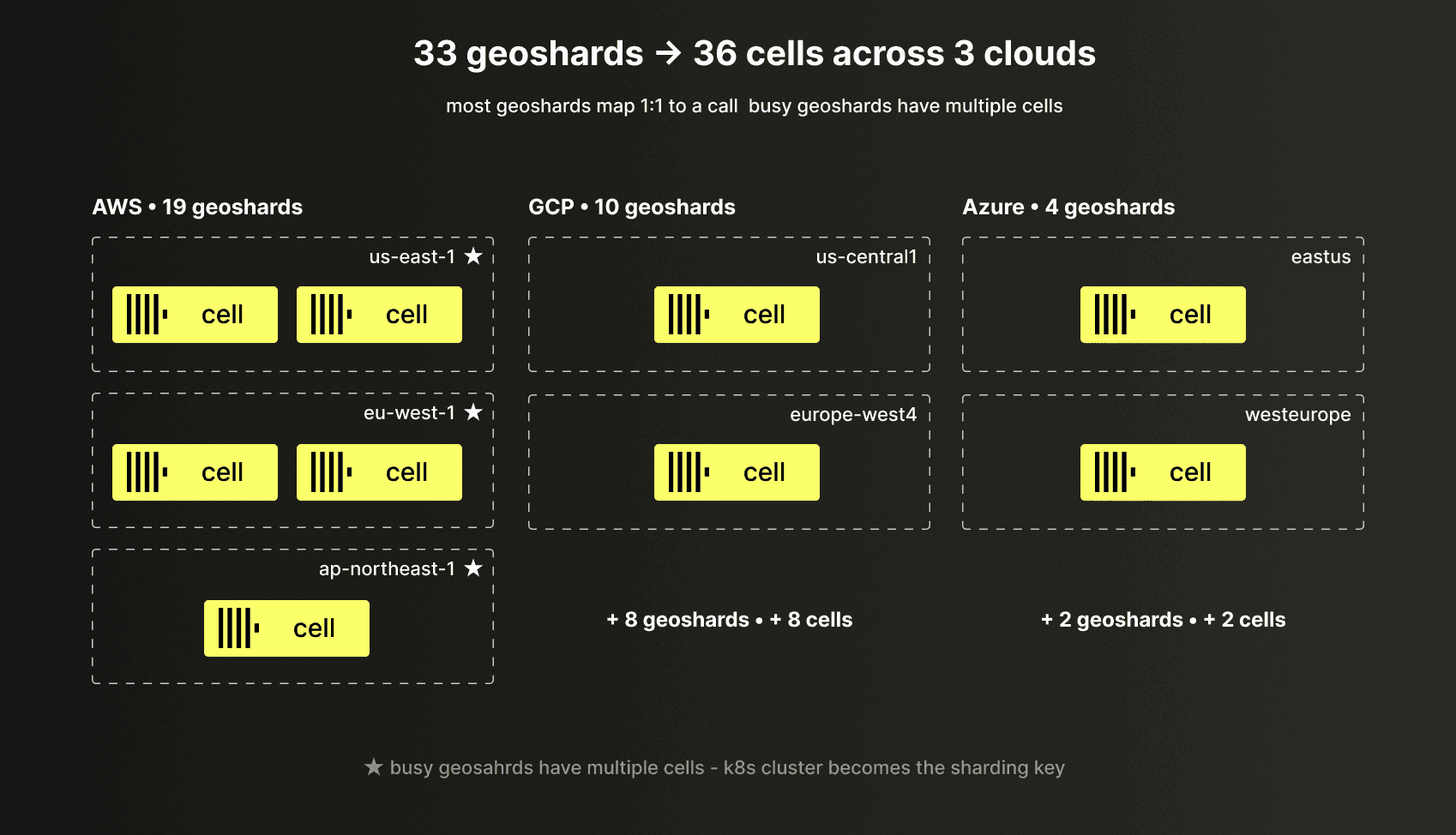
LogHouse now runs on 33 geoshards (36 cells in total) across three cloud providers, with each cell a separate ClickHouse Cloud instance. Most geoshards consist of a single cell, but our busiest regions have multiple cells.

At peak, the system ingests:

• 80 GiB/s of uncompressed data
• 190 million rows per second
• across ~5,800 inserts per second

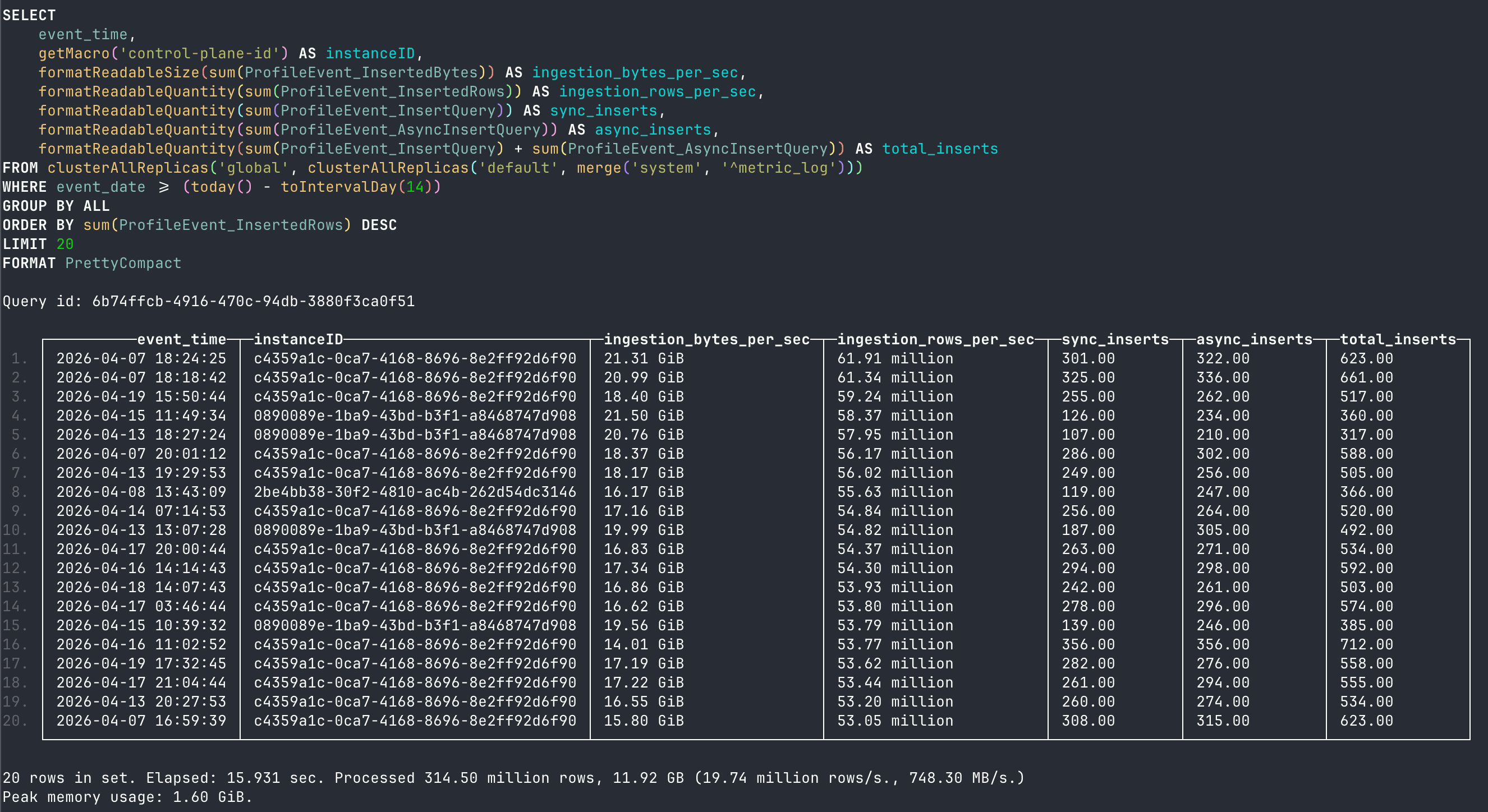
Our busiest single cell handles 21 GiB/s, 61 million rows per second, and 620 inserts per second at peak.

Why we created cells

The first is blast radius. When something goes wrong with a cell (ClickHouse cluster), only the logs flowing through it are affected. The rest of the region keeps writing and reading normally. With a single cell per region, every operational issue would take out the entire region's visibility.

The second is alignment with the data plane. ClickHouse Cloud itself is already organized into cells underneath, and our logging infrastructure can mirror that structure. This lets us place each LogHouse cell in a Kubernetes cluster with predictable, evenly distributed load, rather than forcing one Kubernetes cluster to absorb all of a region's logging traffic.

Isolated cell writes

When one cell isn't enough for a region, we add more within it and use the source Kubernetes cluster as the secondary sharding key. Nothing stops us from creating even more cells, with some additional work on the client side. The result is 36 independent ClickHouse clusters writing in parallel, with no contention point anywhere on the path.

Taming the small-writes problem with Async Inserts

Always-local cell creation solves scaling. It also walks us straight into the failure mode every ClickHouse user eventually meets. We have hundreds of writers (SysEx scrapers, OTel collectors, data-plane services), all sending data continuously, most of it in small chunks. Point this at ClickHouse naively, and each synchronous insert becomes its own data part: thousands of tiny parts per second. Each new part means a metadata update in ClickHouse Keeper, network traffic to flush data, and merge pressure to consolidate small parts into larger ones. The merge scheduler falls behind, and ClickHouse eventually rejects writes outright with a TOO_MANY_PARTS error.

The official guidance is to batch at least 10,000–100,000 rows and insert no more than about once per second per table. But asking hundreds of producers to buffer batches that large locally is impractical: the data is time-sensitive, and if a collector crashes, whatever it was holding is lost.

Async Inserts solve this directly. Instead of each small insert immediately creating a new data part on disk, ClickHouse accumulates incoming rows into server-side buffers. When a buffer reaches a configured threshold (a time limit or a data size limit), the accumulated rows are flushed together as a single, well-sized part.

Here's what that looks like for two of our busiest tables during a peak hour on our heaviest cell.

otel_logs

text_log

Writer

OTel collectors

SysEx scrapers

Client insert size

~8 MiB, low variance

highly variable — 23 MiB p50, 696 MiB p99

Client inserts / hour

290,284

74,373

Parts created / hour

12,082

18,197

Batching ratio

~24×

~4×

Resulting part size

195 MiB / 178K rows

311 MiB / 911K rows

otel_logs is the canonical case Async Inserts were designed for: a steady stream of ~8 MiB writes from hundreds of OTel collectors. Roughly 24 of these get coalesced into each part, collapsing the part-creation rate by more than an order of magnitude.

text_log is shaped very differently. Our SysEx scrapers already aggressively batch before sending, ranging from 23 MiB to nearly 700 MiB per request. We deliberately don't push client-side batching further, because larger buffers on the scraper side would mean significant memory pressure and a non-trivial amount of infrastructure rework. So the batching ratio is a more modest 4×. But even 4× is a big win at this scale: the difference between 74,373 and 18,197 parts per hour on a single table on a single cell, which works out to roughly 56,000 fewer part-creation entries in Keeper every hour and 56,000 fewer items for the merge scheduler to process.

The writer shapes are very different, but the outcome is the same: parts land in the 195–311 MiB range at 178K–911K rows each.

Choosing the right partition key

As the partitioning best practices guide explains, partitioning in ClickHouse is primarily a data management technique. It controls how data is organized on disk, how TTL policies drop old data, and how parts are merged, since ClickHouse only merges parts within the same partition, never across partitions. The key constraint is cardinality: the guide recommends fewer than 100–1,000 distinct partition values to keep part counts manageable.

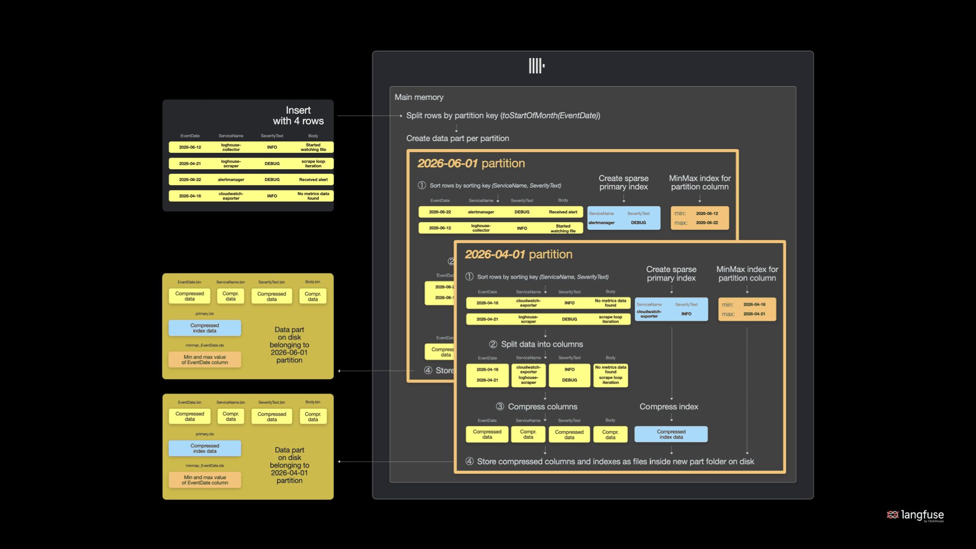
Example partitioning strategy. See the documentation for a more detailed explanation.

Most of our SysEx tables are partitioned by month. With a 180-day or 365-day TTL, this produces 6 to 12 active partitions at any time, well within the recommended range, and it aligns cleanly with retention policies.

For our largest tables, such as text_log, monthly partitions became a problem, and it took us a while to see exactly why. It wasn't that merges were too slow. On the largest tables, a single month accumulated a large number of parts that had already reached the maximum merged part size (150GB), so ClickHouse stops further merging. That size is itself a setting we could raise — but larger parts would hurt read performance, so merging our way out isn't the answer. The part count just kept climbing within the month, walking us towards the too-many-parts ceiling.

To solve this, we switched from monthly to daily partitioning. With a 180-day TTL, this gives us ~180 active partitions, still comfortably within the recommended cardinality range. Each partition receives fewer inserts, parts stay smaller and more manageable, and merges keep up. TTL drops are also cleaner since ClickHouse can drop an entire day's partition in a single metadata operation. The tradeoff is that queries spanning long time ranges now touch more partitions, but in practice, LogHouse users mostly filter by a narrow time window, so this is rarely an issue.

Reliable delivery for OTel data

In our previous post, we described SysEx's pull-based model and how it naturally handles backfill and avoids data loss. Our OTel pipeline (which still handles 95 PiB and 109 trillion rows) needed its own reliability story.

Async Inserts and partitioning got us a long way, but they don't help with the harder problem: what happens when the target ClickHouse cell itself is unavailable? Collectors have limited in-memory buffers, and logs keep coming whether we're ready for them or not.

The default OpenTelemetry behavior when an insert fails is to buffer the batch in memory and retry. That's how our pipeline started out: collectors held failed batches in memory while a Horizontal Pod Autoscaler (HPA) added replicas to handle growing memory pressure. The problem was capacity. The in-memory buffer is bounded by pod memory, and HPA scale-up takes time - a long enough LogHouse outage could outrun both.

So we layered S3 underneath. Collectors still buffer failed batches in memory by default, but when memory runs low, the buffer spills to an S3 bucket — a persistent, effectively unbounded backstop. A background process drains that bucket, retrying batches against LogHouse as soon as the cell is healthy again. Once a batch is safely inserted, it's removed from S3.

A LogHouse outage becomes an ingestion delay instead of data loss. The in-memory buffer absorbs short interruptions, S3 catches the long tail, and ClickHouse picks up the backlog on its own schedule once it recovers. We trade a small amount of write latency for a much calmer failure mode: when the pipeline isn't healthy, collectors don't crash, don't drop data, and don't require manual intervention to recover.

Async Inserts, daily partitioning, and the S3 fallback weren't single heroic fixes — they're points on a curve we keep adjusting. We tune the write path continuously: an Async Insert threshold here, a partition key there, an index dropped once it stopped earning its place.

Cross-cloud, cross-regional distributed queries with low latency

Before any of this, reading LogHouse meant knowing where your data lived. Each region was a separate ClickHouse instance with its own FQDN, and LogHouse users connected to whichever region they cared about directly, through clickhouse-client or as a per-region Grafana data source. Even at a dozen regions, this was awkward to manage and to use, but it was about to get worse: the moment we split a busy region into multiple cells, a user would have to know not just which region held their data but which cell within it. That was the line we didn't want to cross.

So we introduced Distributed tables before we added a second cell to any region — they were the prerequisite for cell creation, not a consequence of it. The goal was a single endpoint that hides the topology entirely: users query one table, and the routing happens underneath.

These tables also made ClickStack much easier to use. For some time, we had wanted to move more of our internal observability workflows into the ClickStack UI. Previously, Grafana relied on region-aware routing, requiring users to select a specific regional data source before querying data. Replicating that model and UI logic in a general-purpose observability interface was impractical. Distributed tables removed that complexity, allowing users to query data across regions through a single logical data source.

A three-level table hierarchy

Achieving this required more than just a single endpoint. We needed a hierarchy that could hide cells and regions from users, while preserving efficient routing and allowing the topology underneath to evolve over time.

We solved this with a three-level table structure, all using the same schema deployed identically across every cell.

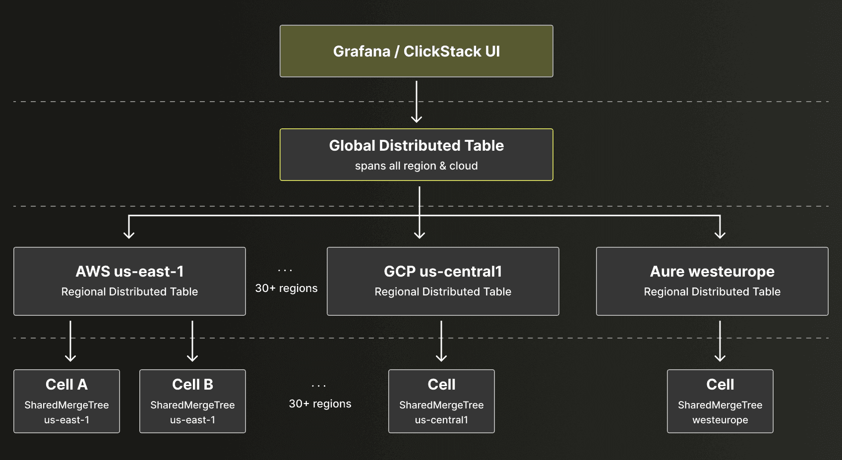
Distributed tables are a virtual federation layer that sit above physical tables and cells. In LogHouse, they provide a stable query endpoint that transparently routes requests across cells and regions. While shown as a single logical layer in the diagram, Distributed tables contain no data themselves and must be created on every ClickHouse node.

At the bottom sits the actual data in a SharedMergeTree table, for example, otel.generic_logs_0.

Above it, a regional Distributed table (otel.generic_logs_region) references a regional cluster. This cluster lists only the cells within the local region, addressed as Kubernetes Services, so traffic never leaves the Kubernetes cluster and there's no Istio or NLB overhead.

At the top, a global Distributed table (otel.generic_logs) references a global cluster. This cluster lists every region, addressed via Istio endpoints (the same load balancers that ClickHouse Cloud customers use). Critically, the shard_name in this cluster config is set to the region name. This becomes important for shard pruning.

-- Level 1: global — spans all regions and clouds
otel.generic_logs
  Engine: Distributed('global', 'otel', 'generic_logs_region', sharding_key)

-- Level 2: regional — spans cells within one region
otel.generic_logs_region
  Engine: Distributed('regional', 'otel', 'generic_logs_0')

-- Level 3: local — the actual data
otel.generic_logs_0
  Engine: SharedMergeTree

This hierarchy makes it easy to add new regions (add an entry to the global cluster config) or add cells to a hot region (add entries to that region's regional cluster config), all without changing the tables that LogHouse users query. The Distributed tables serve as a stable API contract: users always query the global table, and the routing happens transparently.

Each cell has its own unique remote_servers config. The local region and cell are always represented as localhost, so queries that don't need to leave the region never touch the network.

Beyond hiding the topology, the Distributed engine buys us two things that matter at this scale.

Firstly, they keep a persistent connection pool to all cells, eliminating DNS resolution, TLS handshakes, and connection setup on every query. This is significant when you're querying across 36 cells.

Secondly, they have built-in retry logic: when a connection to a remote cell fails due to a transient network issue or a stale pooled connection, the engine retries using a fresh one. This is essential when transient failures happen regularly across cloud boundaries.

The third piece, sharding key support, is what actually keeps SELECT latency low, and it gets its own section next.

Keeping queries fast with optimize_skip_unused_shards

Most LogHouse queries look something like: "show me logs for namespace X in region Y over the last hour." Time and namespace are handled by partitioning (EventDate) and the primary key (Namespace, EventTime). But what about region?

A single global Distributed table is easy to make correct and easy to make slow. Left alone, it would answer every query by fanning out to all 36 cells and waiting for the slowest to respond, even when the data lives entirely in one region. That tail is the whole problem: every cross-region hop is another place a stale connection or slow cell could wreck the p99.

The solution is ClickHouse's optimize_skip_unused_shards setting combined with a sharding key. If the Distributed table knows which cell holds data for a given region, it can skip all the others.

We didn't want to hand-maintain that region→shard mapping; we wanted it to come straight from the cluster topology that ClickHouse already knows about. A dictionary sourced from system.clusters does exactly this — it lifts the global cluster layout into something we can call as a sharding-key function. It's not the most obvious use of a dictionary, but it's clean, and because we add regions and cells regularly, we let it refresh on a short lifetime so the mapping is never stale:

CREATE DICTIONARY default.regionToShard
(
    `region` String,
    `shardID` Int64
)
PRIMARY KEY region
SOURCE(CLICKHOUSE(
    QUERY 'SELECT shard_name AS region, shard_num - 1 AS shardID
           FROM system.clusters
           WHERE name = ''global'''
))
LIFETIME(MIN 0 MAX 300)
LAYOUT(COMPLEX_KEY_HASHED()

The global Distributed table uses dictGet('default.regionToShard', 'shardID', Region) as its sharding key. Now, when a query includes WHERE Region = 'us-east-1' and optimize_skip_unused_shards is enabled, ClickHouse evaluates the sharding key expression, determines which cell(s) match, and sends the query only there. A query that would have touched 36 cells now touches two.

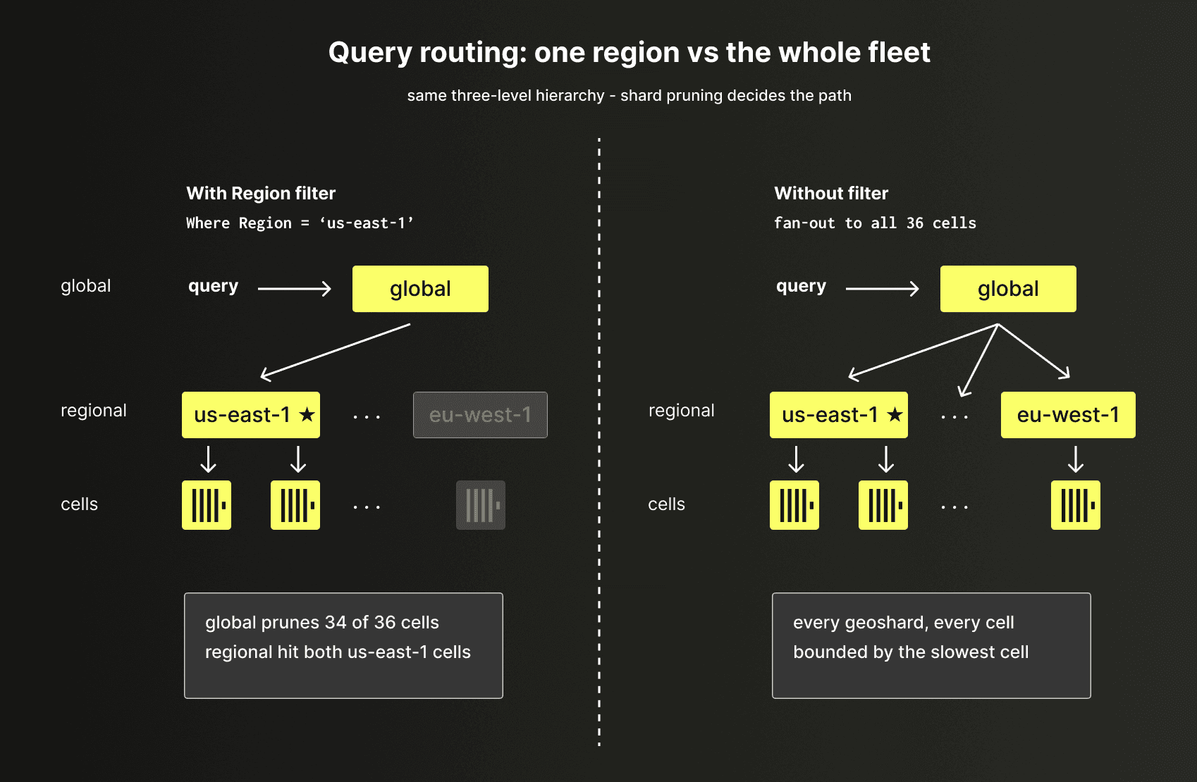
While the same mechanism could be pushed down to the regional level too, pruning within a region's cells, those cells are physically close, and the benefits wouldn't justify the complexity, so we haven't. Region-level pruning is where essentially all the value is.

Latency in practice

To make this concrete, consider a typical query pattern — counting otel-collector errors per region over the last hour:

SELECT
    Region,
    count() AS errors
FROM otel.generic_logs
WHERE (EventDate = today()) AND (EventTime >= (now() - toIntervalHour(1))) AND (SeverityText = 'ERROR') AND (Namespace = 'o11y') AND (PodName LIKE 'loghouse-agent%')
GROUP BY ALL
ORDER BY ALL ASC
SETTINGS force_optimize_skip_unused_shards = 0

    ┌─Region───────────────┬─errors─┐
 1. │ af-south-1           │      3 │
 2. │ ap-east-1            │      2 │
 3. │ ap-northeast-1       │     37 │
 4. │ ap-northeast-2       │      2 │
 5. │ ap-south-1           │     52 │
 6. │ ap-southeast-1       │     42 │
 7. │ ap-southeast-2       │     25 │
 8. │ asia-northeast1      │     14 │
 9. │ asia-southeast1      │     32 │
10. │ australia-southeast1 │      2 │
11. │ australiaeast        │      1 │
12. │ ca-central-1         │      2 │
13. │ eastus2              │      1 │
14. │ eu-central-1         │    169 │
15. │ eu-north-1           │      6 │
16. │ eu-west-1            │    218 │
17. │ eu-west-2            │     53 │
18. │ eu-west-3            │      1 │
19. │ europe-west2         │      4 │
20. │ europe-west3         │      1 │
21. │ europe-west4         │    194 │
22. │ germanywestcentral   │      9 │
23. │ il-central-1         │      2 │
24. │ sa-east-1            │      1 │
25. │ us-central1          │     79 │
26. │ us-east-1            │    535 │
27. │ us-east-2            │    216 │
28. │ us-east1             │     27 │
29. │ us-west-2            │    260 │
30. │ westus3              │      2 │
    └──────────────────────┴────────┘

29 rows in set. Elapsed: 1.591 sec. Processed 33.39 million rows, 248.34 MB (20.99 million rows/s., 156.13 MB/s.)
Peak memory usage: 299.57 MiB.

Without a Region filter, this fans out to all 36 cells. The query returns rows for 29 regions with errors and completes in about 1.6 seconds, processing 33M rows. That's slower than a typical fleet-wide query, and text_log shows exactly why: the coordinator hit five stale pooled TCP connections, and one of them was to asia-southeast1. A full TCP+TLS handshake to Singapore took roughly 700 ms, after which the Singapore cell needed another ~600 ms to execute and stream back. Local planning, primary-key pruning, and aggregation took only ~75 ms in total — the rest is exactly the tail-latency story we wanted to avoid.

Filtered to the local region (Region = 'us-east-2', where the query was initiated), a similar query to collect errors by component completes in 270 ms, processing 2.7M rows.

SELECT
    LA['component'] AS component,
    count() AS errors
FROM otel.generic_logs
WHERE (EventDate = today()) AND (EventTime >= (now() - toIntervalHour(1))) AND (SeverityText = 'ERROR') AND (Namespace = 'o11y') AND (PodName LIKE 'loghouse-agent%') AND (Region IN ('us-east-1'))
GROUP BY ALL
ORDER BY ALL ASC

 ┌─component────┬─errors─┐
 │              │      3 │
 │ fileconsumer │    612 │
 └──────────────┴────────┘

2 rows in set. Elapsed: 0.831 sec. Processed 9.55 million rows, 240.12 MB (11.48 million rows/s., 288.83 MB/s.)
Peak memory usage: 386.84 MiB.

Filtered to a cross-cloud, cross-continent region (Region = 'europe-west4'), we see ~291 ms — actually faster than the same-cloud query to us-east-1. The cross-continent network hop adds real but modest cost; the dominant factor turns out to be how much data each cell has to scan, and europe-west4 simply had fewer rows (2.81M).